Newton’s method is a root-finding algorithm that can be used to find the roots of differentiable functions. It is a very simple algorithm to implement, and it converges quickly in most cases, of course depending on the function. It is often used to find the roots of polynomials. For instance, in Chemical Engineering properties calculations, often cubic equations of state are used to model the behavior of fluids. These equations of state are cubic polynomials and most solved for their roots in most cases in order to compute fluid properties and phase equilibria. For cubic polynomials, it’s possible to find the roots analytically, it’s also possible to find the roots numerically using Newton’s method. One algorithm that is used sometimes combines both methods as an optimization. It uses Newton’s method to find one real root (will exist for a cubic), and then ‘deflates’ the cubic polynomial into a quadratic polynomial, so that quadratic formula can be used to find the other two roots.

So how does Newton’s Method work in general?

Newton’s Method for Root Finding

Newton’s method comes from a Taylor series expansion of a function around a point. The Taylor series expansion of a function $f(x)$ around a point $x_0$ is given by:

$$ f(x) = f(x_0) + f’(x_0)(x - x_0) + \frac{f’’(x_0)}{2!}(x - x_0)^2 + \frac{f’’’(x_0)}{3!}(x - x_0)^3 + \cdots $$

If we truncate the series at the second term, we get:

$$ f(x) \approx f(x_0) + f’(x_0)(x - x_0) $$

And if we set $f(x) = 0$, we get:

$$ 0 = f(x_0) + f’(x_0)(x - x_0) $$

Solving for $x$ gives us: $$ x = x_0 - \frac{f(x_0)}{f’(x_0)} $$

So we have an iterative method to find the roots of the function $f(x)$, given some initial guess $x_0$. Often convergence is very fast, but it depends on the properties of the function. We’re basically assuming that at small steps, the function is linear, and we’re using that to find the root. There’s also an obvious issue if the derivative goes to zero, and there many adaptations of Newton’s method that improve it for different cases.

Simple Example

Let’s try to find the roots of the function $f(x) = x^2 - 4$ using Newton’s method. We know that the roots of this function are $\pm \sqrt{4}$. All the code is available in this GitHub Gist. First we can define some functions, one evaluates the polynomial and the other evaluates the derivative of the it at any point $x$.

def get_f_df(c: list[int]) -> tuple[callable, callable]:
  """ Get the function and its derivative for a given polynomial c"""

  def f(z):
    ans = 0
    for i, c_i in enumerate(c):
      ans += c_i * z**(len(c) - i - 1)
    return ans
  
  def df(z):
    ans = 0
    for i, c_i in enumerate(c):
      ans += (len(c) - i - 1) * c_i * z**(len(c) - i - 2)
    return ans
  
  return f, df

This is a function that returns f and df, which are the function and its derivative. It’s generalized so that it can be used for any polynomial, but for this example we only care about the polynomial $f(x) = x^2 - 4$. We will use like this:

f, df = get_f_df([1, 0, -4])

And we can then evaluate the function and its derivative at any point $x$:

f(0) # -4
df(0) # 0

Now let’s try to find the roots of the function $f(x) = x^2 - 4$ using Newton’s method. We need to define a function that implements the algorithm:

1. Given an initial guess $x_0$, compute $f(x_0)$ and $f’(x_0)$
2. Compute $x_{n+1} = x_n - \frac{f(x_n)}{f’(x_n)}$
3. Evaluate stopping criteria:
   • if not met, set $x_n = x_{n+1}$, go back to step 2
   • If met, stop. You found a root!

Stopping criteria can be based on the difference between the current and the previous $x$ value, or how close $f(x)$ is to zero, etc. For this example we can just stop when $f(x)$ is close to zero. Here’s the code:

def newton(
    x0: complex,
    f: callable,
    df: callable,
    tol: float=1e-12,
    maxiter: int=100):
  """ Newton's method for solving f(x) = 0 """
  x = x0
  for i in range(maxiter):
    x = x - f(x)/df(x)
    print(f"i: {i}, x: {x}, f(x): {f(x)}")
    if abs(f(x)) < tol:
      return x
  raise("Newton's method did not converge")

Applying this function to our polynomial $f(x) = x^2 - 4$, with initial guess $x_0 = -4$:

i: 0, x: -2.5, f(x): 2.25
i: 1, x: -2.05, f(x): 0.20249999999999968
i: 2, x: -2.000609756097561, f(x): 0.002439396192741583
i: 3, x: -2.0000000929222947, f(x): 3.716891878724482e-07
i: 4, x: -2.000000000000002, f(x): 8.881784197001252e-15

We can see that after 5 iterations, we’re really close to the root $x = -2$. If we start with $x_0 = 4$ instead, we converge to the other root:

i: 0, x: 2.5, f(x): 2.25
i: 1, x: 2.05, f(x): 0.20249999999999968
i: 2, x: 2.000609756097561, f(x): 0.002439396192741583
i: 3, x: 2.0000000929222947, f(x): 3.716891878724482e-07
i: 4, x: 2.000000000000002, f(x): 8.881784197001252e-15

Here’s what it looks like plotted:

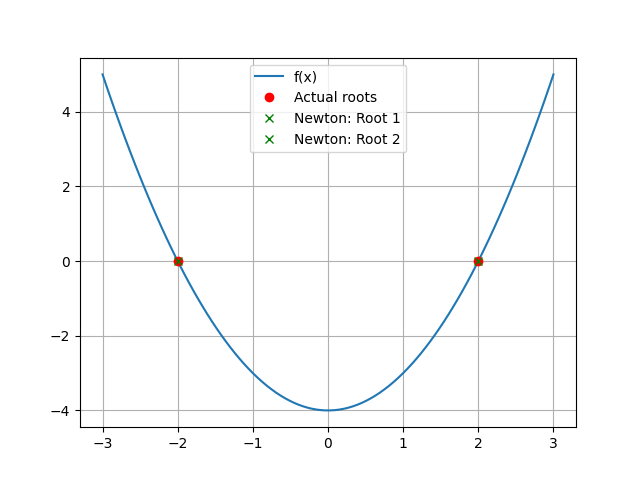
The root we find can be different depending on the initial guess. Sometimes, this behaves intuitively - e.g. we just converge to the root that is closest to the initial guess. This is the case for quadratic polynomials. But for cubics and higher, the situation is different and small changes in the initial guess can lead to very different roots. This is where things get interesting!

Newton Fractals

Let’s say we take our function $f(x) = x^2 - 4$, and we try a bunch of starting points $x_0$ in the complex plane. For each starting point, we apply Newton’s method, and we record whether we converged to root 1 or root 2. If we plot, we see something like this:

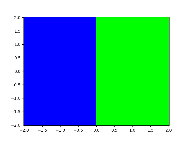
The color of each point represents which root we converged to. We can see that we simply converge to the root that is closest to the initial guess in this case.

But that’s not always the case. Let’s try a different function: $f(x) = x^3 - 1$

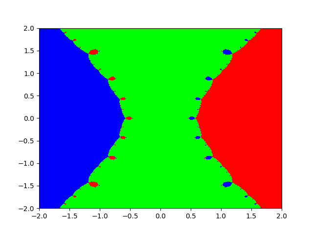
This is a cubic, so there are three roots. We’ll try the same thing, we’ll take a bunch of starting points in the complex plane, and we’ll apply Newton’s method to each one. We’ll record which root we converged to, 1, 2, or 3, and we’ll plot the results for each starting point:

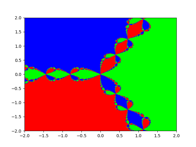
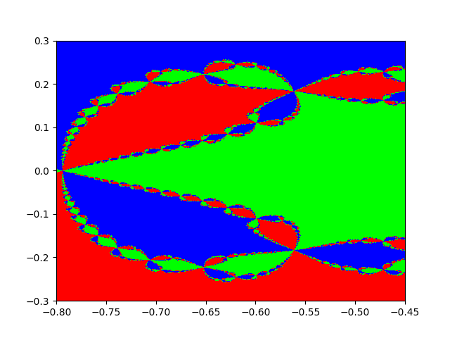
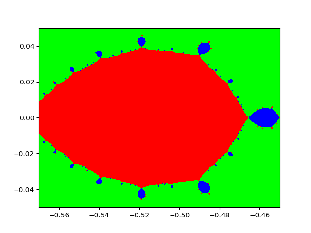
That’s pretty cool! We can see that tiny changes in the initial guess cause our Newton’s method to converge to different roots - and that this pattern produces a fractal. If we keep zooming in, we’ll keep seeing repeating patterns at the boundary. Here’s a zoomed in version of the plot above:

And of course different functions produce different fractals. Here’s another one that’s pretty cool: $f(x) = x^3 - x$:

and zoomed in on one of the little bumps:

That’s pretty mind blowing right?

Anyway, I’ve always thought this we cool and I’ve seen some people posting Mandelbrot fractals - so it reminding of this and I thought I’d share it.

Let me know if you have any questions or comments! Would be cool to make a zooming animation, but unfortunately I think reasonable frame rates would require an ‘anything but Python’ approach 😂

All the code for part two is in this GitHub Gist.

Checkout this 3Blue1Brown on this topic for more details amazing animations.